Forecasting Stock Prices Using Stock Correlation Graph: A Graph Convolutional Network Approach
Published:
IJCNN 2021 · IEEE
Forecasting Stock Prices Using Stock Correlation Graph
基于股票相关性图的股价预测:一种图卷积网络方法Forecasting Stock Prices Using Stock Correlation Graph: A Graph Convolutional Network Approach
Glad to see this work being used by quant firms :)很高兴看到这项研究被量化机构采用 :)
The Problem问题所在
Predicting where a stock price is heading matters for investment, and deep learning models have become a standard tool for it. Almost all of them are built the same way: take one stock's own history — its past prices, sometimes technical indicators or news — and train a sequence model to extrapolate it.预测股价走向对投资很重要,深度学习模型已成为这类任务的标准工具。而这些模型几乎都是同一个套路:拿单只股票自己的历史 —— 它过去的价格,有时再加上技术指标或新闻 —— 训练一个序列模型去外推。
That framing throws away something obvious about markets. Stocks do not move independently. Two companies in the same sector, or two funds holding overlapping assets, tend to rise and fall together. If the model only ever looks at one stock's own past, it cannot use the fact that a related stock has already moved — even though that is exactly the kind of signal a trader would look at.但这个设定丢掉了市场上一件显而易见的事:股票不是各走各的。同行业的两家公司,或持仓高度重叠的两只基金,往往同涨同跌。如果模型只看一只股票自己的过去,它就用不上「相关股票已经动了」这个事实 —— 而这恰恰是交易员一定会看的信号。
So the problem this work addresses is narrow and concrete: existing sequence models leave the information carried by similar stocks unexplored.所以这项工作要解决的问题很窄也很具体:现有序列模型忽略了相似股票所携带的信息。
Key Idea核心思路
The fix is to stop treating each stock as an isolated time series, and instead make the relationships between stocks part of the input.做法是:不再把每只股票当成一条孤立的时序,而是把股票之间的关系本身变成输入的一部分。
Which stocks move together is itself data. Compute it once from historical prices, turn it into a graph, and let every stock's prediction draw on its neighbours.「哪些股票会同涨同跌」本身就是数据。从历史价格里算一次、把它变成一张图,然后让每只股票的预测都能借用邻居的信息。
The graph is built by taking the Pearson correlation of every pair of price sequences and then binarising it with a cutoff τ = 0.9, so that only the strongest links survive. Binarising matters: if every pair stays weakly connected, graph convolution averages everything together and the features become uninformative.图是这样建的:对每一对价格序列求皮尔逊相关系数,再用阈值 τ = 0.9 二值化,只保留最强的连接。二值化这一步很关键:如果每一对股票都保留弱连接,图卷积就会把所有特征平均到一起,特征反而失去信息量。
How It Works方法
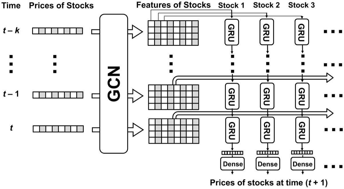
Figure 1: The model. A shared GCN module turns each stock together with its highly correlated neighbours into a feature vector; those feature vectors are fed, in time order, into a per-stock GRU whose output predicts the next price.图 1:模型结构。一个共享的 GCN 模块把每只股票及其高度相关的邻居一起编码成特征向量;这些特征向量按时间顺序送入该股票自己的 GRU,输出即下一时刻的价格预测。
- Build the stock correlation graph. From the training period's prices, compute the correlation matrix over all stocks and keep only edges above the cutoff τ. On the DOW universe this keeps 30.9% of edges; on the ETF universe only 19.8%, because ETFs already share a high base correlation of roughly 0.5 with each other.构建股票相关图。用训练期的价格计算所有股票两两之间的相关矩阵,只保留高于阈值 τ 的边。在 DOW 股票池中保留 30.9% 的边;在 ETF 池中只保留 19.8% —— 因为 ETF 彼此之间本身就有约 0.5 的高基础相关性。
- Extract features with a shared GCN. At each time step the GCN runs over the graph, so a stock's feature vector is built from its own price and the prices of the stocks it is strongly correlated with. One GCN is shared across every stock and every time step.用共享 GCN 提取特征。每个时间步,GCN 在图上运行一次,于是某只股票的特征向量同时来自它自己的价格和与它强相关那些股票的价格。所有股票、所有时间步共用同一个 GCN。
- Predict each stock with its own GRU. The sequence of GCN features for a given stock is fed into that stock's GRU to capture temporal dependence, and a dense layer outputs the next price. All the GRUs are trained together with the shared GCN, following multi-task learning: every stock has its own predictor, but the shared module is trained on all of them at once, which is what lets correlation-related market signals propagate properly through the graph.每只股票用自己的 GRU 做预测。某只股票的 GCN 特征序列送入它自己的 GRU 以捕捉时间依赖,再由一层全连接输出下一价格。所有 GRU 与共享 GCN 一起训练,遵循多任务学习:每只股票各有预测器,但共享模块同时在全部股票上受训 —— 这正是相关性市场信号能够在图上有效传播的原因。
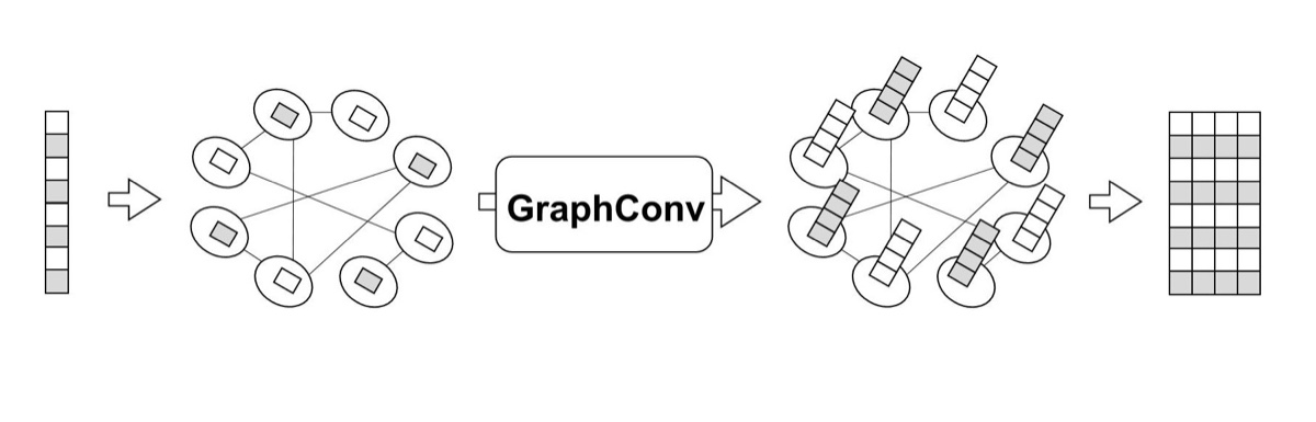
Figure 2: Graph convolution. Each stock aggregates information from the neighbours it is strongly correlated with, so the feature it feeds to its GRU reflects more than its own price history.图 2:图卷积。每只股票从与它强相关的邻居处聚合信息,因此送入 GRU 的特征所反映的,不只是它自己的价格历史。
Results实验结果
The model is compared against a plain GRU baseline that sees only a single stock's price sequence — the same architecture with the graph removed, so any difference comes from using correlated stocks. Experiments use daily price data from 2010-11-22 to 2020-06-04: the first 80% (up to 2018-07-05) builds the correlation graph and trains the models, the rest is held out for testing. The two universes are the 30 Dow Jones stocks and the top 50 ETFs.对比对象是一个只看单只股票价格序列的普通 GRU 基线 —— 同一套架构、只是把图去掉,因此任何差异都来自「使用了相关股票」这一点。实验使用 2010-11-22 至 2020-06-04 的日频价格数据:前 80%(截至 2018-07-05)用于构建相关图并训练模型,其余留作测试。两个股票池分别是 30 只道琼斯成分股和前 50 只 ETF。
Table 1: Our model versus the GRU baseline on 6 DOW stocks and 4 ETFs. "Accuracy" is price-direction classification; "Accuracy\*" is ε-insensitive accuracy, which does not count a prediction as wrong when the predicted price is within ε = $0.2 of the previous price. Best result in each pair is bold.表 1:本文模型与 GRU 基线在 6 只 DOW 股票与 4 只 ETF 上的对比。「Accuracy」为价格方向分类准确率;「Accuracy\*」为 ε-不敏感准确率 —— 当预测价格与上一价格之差在 ε = $0.2 以内时不计为错误。每组中更优的结果加粗。
| Stock | Model | Accuracy | Accuracy* | R² | RMSE | MAE | RE |
|---|---|---|---|---|---|---|---|
| AA | GRU | 0.5400 | 0.6178 | 0.9885 | 0.8748 | 0.7403 | 0.0415 |
| AA | Ours | 0.5332 | 0.6545 | 0.9918 | 0.6228 | 0.5258 | 0.0282 |
| AIG | GRU | 0.5011 | 0.5606 | 0.9825 | 1.2375 | 0.8064 | 0.0219 |
| AIG | Ours | 0.4897 | 0.5812 | 0.9875 | 1.0443 | 0.6980 | 0.0191 |
| GE | GRU | 0.4691 | 0.7140 | 0.9553 | 0.3751 | 0.2764 | 0.0318 |
| GE | Ours | 0.5057 | 0.7666 | 0.9630 | 0.3416 | 0.2484 | 0.0287 |
| T | GRU | 0.5423 | 0.6018 | 0.8290 | 1.5636 | 1.0971 | 0.0321 |
| T | Ours | 0.5515 | 0.6888 | 0.8767 | 1.3278 | 0.8952 | 0.0259 |
| WBA | GRU | 0.4966 | 0.4989 | 0.9583 | 2.0606 | 1.3332 | 0.0228 |
| WBA | Ours | 0.4966 | 0.5355 | 0.9756 | 1.5750 | 1.0629 | 0.0186 |
| XOM | GRU | 0.5217 | 0.5240 | 0.7459 | 5.5159 | 4.0886 | 0.0731 |
| XOM | Ours | 0.5195 | 0.5584 | 0.8544 | 4.1763 | 2.3925 | 0.0496 |
| EEM | GRU | 0.5059 | 0.5216 | -0.1335 | 2.8253 | 2.2704 | 0.0543 |
| EEM | Ours | 0.5235 | 0.5431 | 0.1770 | 2.4073 | 1.8982 | 0.0454 |
| EWZ | GRU | 0.4706 | 0.5569 | 0.9790 | 0.9790 | 0.6599 | 0.0192 |
| EWZ | Ours | 0.4608 | 0.5765 | 0.9806 | 0.9102 | 0.6423 | 0.0187 |
| XME | GRU | 0.5431 | 0.5804 | 0.9848 | 0.5478 | 0.4156 | 0.0167 |
| XME | Ours | 0.5353 | 0.6824 | 0.9872 | 0.5031 | 0.3736 | 0.0149 |
| XRT | GRU | 0.5137 | 0.5471 | 0.8367 | 1.8077 | 1.2016 | 0.0277 |
| XRT | Ours | 0.5157 | 0.6039 | 0.8885 | 1.4936 | 0.9630 | 0.0218 |
What the numbers say这些数字说明了什么
- Adding the graph helps, and it helps almost everywhere. The ε-insensitive accuracy improves on all 10 products, by 2.0 points at the low end (EWZ) and 10.2 points at the high end (XME). The gain comes from the correlation graph and nothing else — the baseline is the same architecture with the graph removed.加图有用,而且几乎处处有用。ε-不敏感准确率在 10 个标的上全部提升,最低 +2.0 个百分点(EWZ),最高 +10.2 个百分点(XME)。这个增益只能归功于相关图,别无其他 —— 基线就是同一套架构、把图去掉。
- Regression improves consistently, not just on average. R², RMSE, MAE and relative error all improve on all 10 products. Mean R² rises from 0.8126 to 0.8682, and mean relative error falls from 0.0341 to 0.0271.回归指标是一致改善,而不只是平均改善。R²、RMSE、MAE 与相对误差在 10 个标的上全部变好。平均 R² 从 0.8126 升到 0.8682,平均相对误差从 0.0341 降到 0.0271。
- Plain direction accuracy is a misleading metric here. Both models sit near 50% on it, and the baseline sometimes wins. The reason is that daily prices barely move: if the price is $60 today and the model predicts $59.9 rather than $60.1, the direction is scored wrong even though the price is essentially right. That is exactly why the ε-insensitive metric is reported alongside it, and why the gap only shows up there.「纯方向准确率」在这里是个会误导人的指标。两个模型都在 50% 附近,基线有时还更高。原因是日频价格几乎不动:今天 60 块,模型预测 59.9 而不是 60.1,方向就算判错 —— 尽管价格基本是对的。这正是要同时报告 ε-不敏感指标的原因,也是差距只在那里显现的原因。
- The cutoff is a real hyper-parameter. τ = 0.9 gave the best accuracy for almost all stocks. Too low and graph convolution over-smooths; too high and genuinely correlated stocks stop contributing.阈值是个实打实的超参数。τ = 0.9 对几乎所有股票都给出最佳准确率。阈值太低,图卷积会过度平滑;太高,真正相关的股票就不再贡献信息。
Code代码
The implementation is released at github.com/troyyxk/gcgru_stock_prediction, written with TensorFlow, pandas, NumPy, scikit-learn and configparser. Training runs with python3 train.py; the hyper-parameters live in config.ini (learning rate 10−3 with Adam, sequence length k = 60 days, GCN output width 128, batch size 128, 100 epochs). The price data and the adjacency matrix follow a parallel directory layout, so switching dataset or time duration means changing one matching pair of paths.实现已开源在 github.com/troyyxk/gcgru_stock_prediction,基于 TensorFlow、pandas、NumPy、scikit-learn 与 configparser。训练只需运行 python3 train.py;超参数位于 config.ini(学习率 10−3、Adam 优化器、序列长度 k = 60 天、GCN 输出维度 128、batch size 128、100 个 epoch)。价格数据与邻接矩阵采用平行的目录结构,因此切换数据集或时间粒度,只需改一对相互匹配的路径。
Citation引用
If you find this work useful, please consider citing it:如果这项工作对您有帮助,欢迎引用:
@inproceedings{yin2021forecasting,
  title     = {Forecasting Stock Prices Using Stock Correlation Graph:
               A Graph Convolutional Network Approach},
  author    = {Yin, Xingkun and Yan, Da and Almudaifer, Abdullateef and
               Yan, Sibo and Zhou, Yang},
  booktitle = {2021 International Joint Conference on Neural Networks (IJCNN)},
  pages     = {1--8},
  year      = {2021},
  doi       = {10.1109/IJCNN52387.2021.9533510}
}
The published version is available on IEEE Xplore.正式发表版本见 IEEE Xplore。